Phonon Monte Carlo
FreePATHS is a free and open-source implementation of phonon Monte Carlo algorithm. It simulates trajectories of phonons in 3D models of nanostructures, which consists of a box with holes or pillars of various shapes. The algorithm outputs phonon trajectories, heat fluxes, temperature maps and profiles, the thermal conductivity, scattering maps and statistics and other information.
Algorithm
The algorithm runs the simulations step-by-step and phonon-by-phonon. For each phonon, the algorithm calculates trajectory, with a timestep $dt$ and for as many timesteps as required for the phonon to reach the cold side or until a maximum number of timesteps is reached.
Initialization
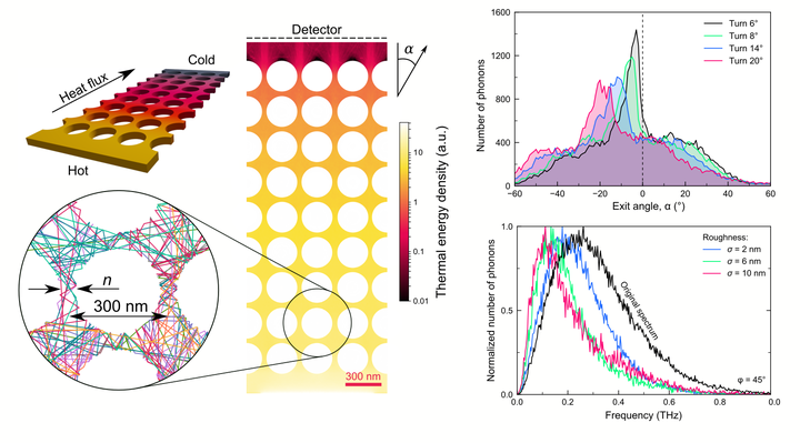
At the beginning of time, each phonon is generated at the hot side. At the this moment, each phonon is assigned a frequency (wavelength) in the and random direction. The frequency is assigned according to the Plank distribution of phonon frequencies at this temperature (T). See the picture above for the example of the Plank distribution function. From the assigned frequency, algorithm determines the phonon group velocity (v) from the phonon dispersion in the given material.
The phonon starts moving step-by-step in the assigned direction according to the following equations:
$\Delta x = sin(\theta)·abs(cos(\phi))·v·dt$
$\Delta y = cos(\theta)·abs(cos(\phi))·t·dt$
$\Delta z = sin(\phi)·v·dt$
where $\theta$ is the angle between the projection to x-y plane and y-axis, and $\phi$ is the angle to the horizontal plane.
Scattering on boundaries
At each time step $dt$, algorithm checks if phonon crossed any of the boundaries. The boundaries include top and bottom of the simulation, left and right walls, or walls of the holes or pillars. If the boundary is crossed, the corresponding function calculates at which angle a phonon hits the boundary. Then, algorithm calculates the specular scattering probability, determined by Soffer’s equation:
$p = exp(-16 \pi ^2 \sigma^2 cos^2(\alpha) / \lambda ^2) $
where $p$ is the specularity probability (number between zero and one), $\sigma$ is the surface roughness, $\alpha$ is the angle to the surface, and $\lambda$ is the wavelength of the phonon. Then the algorithm draws a random number between zero and one. If the number is greater than $p$ than the scattering is diffuse, otherwise specular. If the scattering is specular, the phonon is reflected elastically, from the surface. If the scattering is diffuse, the phonon is reflected in a random direction, but using the Lambert cosine distribution of probability. After the scattering, phonon continues the movement and keeps moving and being scattered until it either reaches the cold side, or returns to the hot side, or time of the simulation for each phonon is over.
Internal scattering
Beside the surface scattering, phonon can also experience internal scattering. The internal scattering includes all resistive scattering processes like impurity scattering, phonon-phonon scattering. In the simulation, this kind of scattering programmed to occur when certain time (relaxation time) passed since last scattering of any kind. In other words, if phonon runs for too long without any scatterings, it’s getting more and more likely to be scattered due to phonon-phonon process. The relaxation time is calculated depending on the phonon frequency, temperature, and polarization.
Distributions and statistics
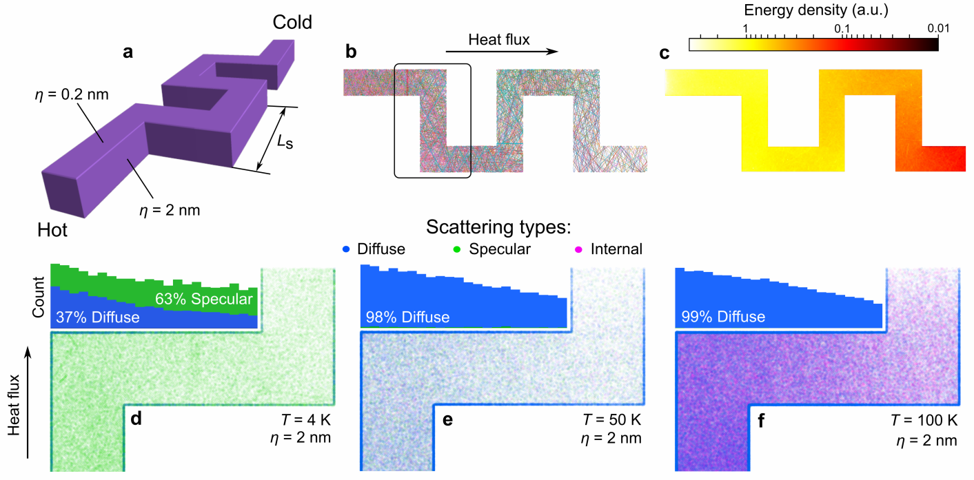
Once the simulation is over for a given phonon, the algorithm collects all the phonon properties (frequency, speed, path etc), it’s entrance and exit angles, and other results and stores it in files. Then, the process repeats for required number of phonons. After simulations for all phonons is done, the algorithm calculates various distributions and statistical facts about the simulation. For example, it calculates phonon spectrum at the beginning, phonon trajectories, phonon exit angle distribution, group velocities etc.. The examples of the distribution are shown above in the picture. Then, it outputs all this information into the graphs and into files. Examples below shows scatterig maps and statistics obtained using the Monte Carlo code for a serpentine nanowire serpentine nanowire.
Acknowledgments
Credits
The code has been developed by Roman Anufriev in Nomura lab at the University of Tokyo since 2018. If you would like to use this code for your research, please cite the papers below, if it is appropriate.
Grants
Development of this code was funded by the following grants:
- PRESTO JST (No. JPMJPR19I1)
- CREST JST (No. JPMJCR19Q3)
- Kakenhi (15H05869, 15K13270, and 18K14078)
- Postdoctoral Fellowship program of Japan Society for the Promotion of Science.
References
- FreePATHS - website of the simulatior
- Singh et al. Applied Physics Letters, (2023)
- Anufriev et al. Materials Today Physics 15, 100272 (2021)
- Anufriev et al. Nanoscale, 11, 13407-13414 (2019)
- Huang et al. ACS Applied Materials & Interfaces 12, 25478 (2020)
- Anufriev et al. ACS Nano 12, 11928 (2018)